Applicability of the Quasistatic Approach to the Calculation of the Characteristics of an Accelerating Towed System
- PDF / 569,830 Bytes
- 6 Pages / 595.276 x 790.866 pts Page_size
- 72 Downloads / 301 Views
International Applied Mechanics, Vol. 56, No. 3, May, 2020
APPLICABILITY OF THE QUASISTATIC APPROACH TO THE CALCULATION OF THE CHARACTERISTICS OF AN ACCELERATING TOWED SYSTEM
Yu. I. Kalyukh
Numerical results of dynamic and quasi-static modeling of the “fast” and “slow” transient processes in towed systems (TS) during the acceleration of their inboard end are compared with experimental data. It is concluded that it is possible to apply the direct dynamic approach to calculating the force characteristics of TS in slow and fast non-stationary processes and the quasistatic approach to calculating the forces. The quasistatic modeling of the geometric characteristics of TS can lead to errors. Keywords: dynamic modeling, quasistatic modeling, accelerated motion, towed system 1. Introduction. To calculate the force characteristics of towed systems (TS) during steady-state motion and during transients, use is made of the quasistationary approach involving the integration of the static equations of a filament in a flow [3, 4, 11]. While there are many theoretical and experimental data on steady-state configurations of rope systems, which suggest its applicability [6], such data are scarce as regards the modeling of “slow” transients in rope systems [1, 2, 7, 9] and practically absent for “fast” transients [5, 8, 10]. Our goal here is to compare numerical results of dynamic and quasistatic numerical simulation of fast and slow transients in a TS with accelerating inboard end and experimental data. 2. Comparative Analysis of Experimental and Numerical Data on the Horizontal Component of the Axial Force at the Inboard End. To analyze the nonstationary stress–strain state (SSS) of a TS consisting of a kapron line and a spherical body at its end, we use the nonlinear dynamic model of a cable in a flow [5]. The system of equations describing the nonstationary behavior of the TS in a plane can be represented in a matrix form: E
¶W ¶W +B = D, ¶t ¶S
(1)
where E is a unit 4´4 matrix; B is the 4´4 matrix in the convective terms; D is the column vector of the right-hand sides; W is the column vector of unknowns. For B, D, and W, we have æ -u t ç ç 1+ eT ç -u n ç B x = ç 1+ eT ç -1 ç e ç ç 0 è
-u n 1+ eT ut 1+ eT
-1 m 0
0
0
-1 1+ eT
0
ö ÷ ÷ u t2 + u n2 T - Mu t2 ÷ ÷ 1+ eT m+ M ÷ , un ÷ e ÷ -u t ÷ ÷ ø 1+ eT 0
State Enterprise “State Research Institute of Building Constructions,” 5/3 Preobrazhenskaya St., Kyiv, Ukraine 03037; e-mail: [email protected]. Translated from Prikladnaya Mekhanika, Vol. 56, No. 3, pp. 138–144, May–June 2020. Original article submitted February 22, 2019. 382
1063-7095/20/5603-0382 ©2020 Springer Science+Business Media, LLC
7 6
5 3
4
1
Fig. 1
pk f rd 0 æ -1 ö ç ( wsinj + ÷ 1+ eT |u t |u t ) 2 çm ÷ ç -1 ÷ k rd Dx = ç ( wcos j + n 0 1+ eT |u n |u n ) ÷ , 2 ç m+ M ÷ ç ÷ 0 ç ÷ 0 è ø
æ ut ö ç ÷ çu ÷ W =ç n ÷ , T ç ÷ çj ÷ è ø
(2)
where d 0 is the initial (before deformation) diameter of the TS; j is the angle between the TS and the horizontal; m, M , w are the mass, added mass, and buoyancy pe
Data Loading...