Binary Logistic Regression
Binary responses are commonly studied in many fields. Examples include 1 the presence or absence of a particular disease, death during surgery, or a consumer purchasing a product. Often one wishes to study how a set of predictor variables X is related to
- PDF / 1,517,972 Bytes
- 56 Pages / 504.581 x 719.997 pts Page_size
- 32 Downloads / 475 Views
Binary Logistic Regression
10.1 Model Binary responses are commonly studied in many fields. Examples include the presence or absence of a particular disease, death during surgery, or a consumer purchasing a product. Often one wishes to study how a set of predictor variables X is related to a dichotomous response variable Y . The predictors may describe such quantities as treatment assignment, dosage, risk factors, and calendar time. For convenience we define the response to be Y = 0 or 1, with Y = 1 denoting the occurrence of the event of interest. Often a dichotomous outcome can be studied by calculating certain proportions, for example, the proportion of deaths among females and the proportion among males. However, in many situations, there are multiple descriptors, or one or more of the descriptors are continuous. Without a statistical model, studying patterns such as the relationship between age and occurrence of a disease, for example, would require the creation of arbitrary age groups to allow estimation of disease prevalence as a function of age. Letting X denote the vector of predictors {X1 , X2 , . . . , Xk }, a first attempt at modeling the response might use the ordinary linear regression model E{Y |X} = Xβ,
(10.1)
since the expectation of a binary variable Y is Prob{Y = 1}. However, such a model by definition cannot fit the data over the whole range of the predictors since a purely linear model E{Y |X} = Prob{Y = 1|X} = Xβ can allow Prob{Y = 1} to exceed 1 or fall below 0. The statistical model that is generally preferred for the analysis of binary responses is instead the binary logistic regression model, stated in terms of the probability that Y = 1 given X, the values of the predictors:
© Springer International Publishing Switzerland 2015
F.E. Harrell, Jr., Regression Modeling Strategies, Springer Series in Statistics, DOI 10.1007/978-3-319-19425-7 10
219
1
220
10 Binary Logistic Regression
Prob{Y = 1|X} = [1 + exp(−Xβ)]−1 .
2
(10.2)
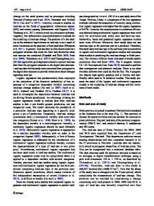
As before, Xβ stands for β0 + β1 X1 + β2 X2 + . . . + βk Xk . The binary logistic regression model was developed primarily by Cox129 and Walker and Duncan.647 The regression parameters β are estimated by the method of maximum likelihood (see below). The function (10.3) P = [1 + exp(−x)]−1 is called the logistic function. This function is plotted in Figure 10.1 for x varying from −4 to +4. This function has an unlimited range for x while P is restricted to range from 0 to 1. 1.0 0.8
P
0.6 0.4 0.2 0.0 −4
−2
0
2
4
X
Fig. 10.1 Logistic function
For future derivations it is useful to express x in terms of P . Solving the equation above for x by using 1 − P = exp(−x)/[1 + exp(−x)]
(10.4)
yields the inverse of the logistic function: x = log[P/(1 − P )] = log[odds that Y = 1 occurs] = logit{Y = 1}. (10.5)
3
Other methods that have been used to analyze binary response data include the probit model, which writes P in terms of the cumulative normal distribution, and discriminant analysis. Probit regression, although assuming a similar shape to the logistic fun
Data Loading...