Moment-based Modeling of Extended Defects for Simulation of TED: What Level of Complexity is Necessary?
- PDF / 279,764 Bytes
- 6 Pages / 420.48 x 639 pts Page_size
- 82 Downloads / 367 Views
INTRODUCTION
It is now well understood that interstitial aggregates, namely {311} defects and dislocation loops, play the central role in transient enhanced diffusion (TED). The formation, evolution and transformation of these defects determine the movement of the dopant. Various models have been proposed for modeling of extended defects. 1 2',3 These models can be classified as "moment-based" as they evolve some parameters of the extended defect distribution over size, since evolving the whole distribution is computationally very expensive. The simplest model is just to keep track of the number of solute atoms in the defects (1-moment model). A next level of model is where the size (or number of defects) is also a model variable (2-moment model), which allows to account for effects of Ostwald ripening. Yet another level is where the lowest three statistical moments of the extended defect distribution over size are considered (3-moment model). In this paper, we will investigate these models and determine what level of complexity is necessary for different systems.
2.
MOMENT-BASED MODEL FOR EXTENDED DEFECTS
We can model the evolution of an extended defect population by explicitly considering precipitates of different sizes as independent species (f,) and account for their kinetics by considering the attachment and emission of solute atoms. 1 I, the net growth rate from size n to n + 1. ma' be written as:
In = DAn (CAfn
- Cf+I)•
(1)
To reduce the number of solution variables, we follow the moment-based approach4 and keep track of only the moments of the distribution (Mi n= -n= n, where i 0,1, 2). The 2 system of equations is then reduced to: Ot =
I2iI J+
[(n + 1)-
ni] In
n=2
105 Mat. Res. Soc. Symp. Proc. Vol. 532 © 1998 Materials Research Society
(2)
500
•,
400
•
S*
o
60s
*
120s
2 300 S200 100 0
0
200
400
600
800
1000
1200
1400
Defect size (atoms) Fig. 1: Distribution of {311} defect densities over defect sizes and best fit to log-normal distribu5 tion. z 2 = 0.8 has been used in all fits. Data from Pan and Tu. Since no finite number of moments can fully describe a full distribution, we need a closure assumption, which is an assumption about the form of the distribution, f" = fr(n, zi). The zi are parameters of the distribution which can be determined from the moments. The number of moments we need to keep track of equals the number of parameters in the distribution function. If nothing is known about the distribution of extended defects over size space, it is logical to use an energy minimizing closure assumption.4 This results in the following distribution with three parameters: zo exp (-AG'cc/kT + zin + z 2 n2)
(3)
However, for {311} defects and dislocation loops the distribution has been measured experimentally.5 The results suggest that the distribution is roughly log-normal:
f, = z0 exp(-ln(n/z1 ) 2/z 2 )
(4)
When we analyze the data, we find that z 2 is independent of annealing time, and distributions can be approximated by log-normal distributions with z 2 = 0.8 (Fig. 1
Data Loading...